42 data labels excel pie chart

How do you display outside end data labels in Excel? The cell values will now display as data labels in your chart. How do I add data labels to a chart in word? Add data labels You can add data labels to show the data point values from the Excel sheet in the chart. This step applies to Word for Mac only: On the Viewmenu, click Print Layout. Click the chart, and then click the Chart Designtab ... Formatting data labels and printing pie charts on Excel for Mac 2019 ... Here's a work around I found for printing pie charts. Still can't find a solution for formatting the data labels. 1. When printing a pie chart from Excel for mac 2019, MS instructions are to select the chart only, on the worksheet > file > print. Excel is supposed to print the chart only (not the data ) and automatically fit it onto one page.

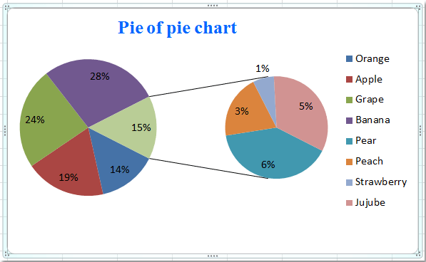
Possible to add second data label to pie chart? - Excel Help Forum You get one data label per plotted point. I think you could use the first trick in this page of Andy Pope's, and make the pie in front the same size as the one in back, and use one pie for the outside labels and the other for the inside labels. - Jon ------- Jon Peltier, Microsoft Excel MVP Peltier Technical Services Tutorials and Custom Solutions

Data labels excel pie chart

How to Make a PIE Chart in Excel (Easy Step-by-Step Guide) Once you have the data in place, below are the steps to create a Pie chart in Excel: Select the entire dataset Click the Insert tab. In the Charts group, click on the 'Insert Pie or Doughnut Chart' icon. Click on the Pie icon (within 2-D Pie icons). The above steps would instantly add a Pie chart on your worksheet (as shown below). Inserting Data Label in the Color Legend of a pie chart Inserting Data Label in the Color Legend of a pie chart. Hi, I am trying to insert data labels (percentages) as part of the side colored legend, rather than on the pie chart itself, as displayed on the image below. Does Excel offer that option and if so, how can i go about it? Multiple Data Labels on a Pie Chart | MrExcel Message Board This table includes: Column 1 - shipment name Column 2 - shipment cost Column 3 - shipment weight I have created a pie chart from this table, which covers the first two columns. Displayed next to each slice is a label with the shipment name, shipment cost, and percent share of the pie.

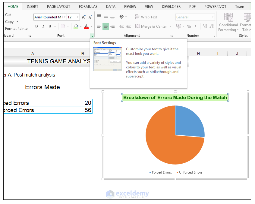
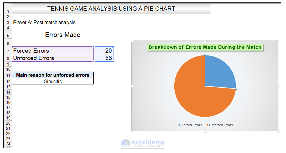
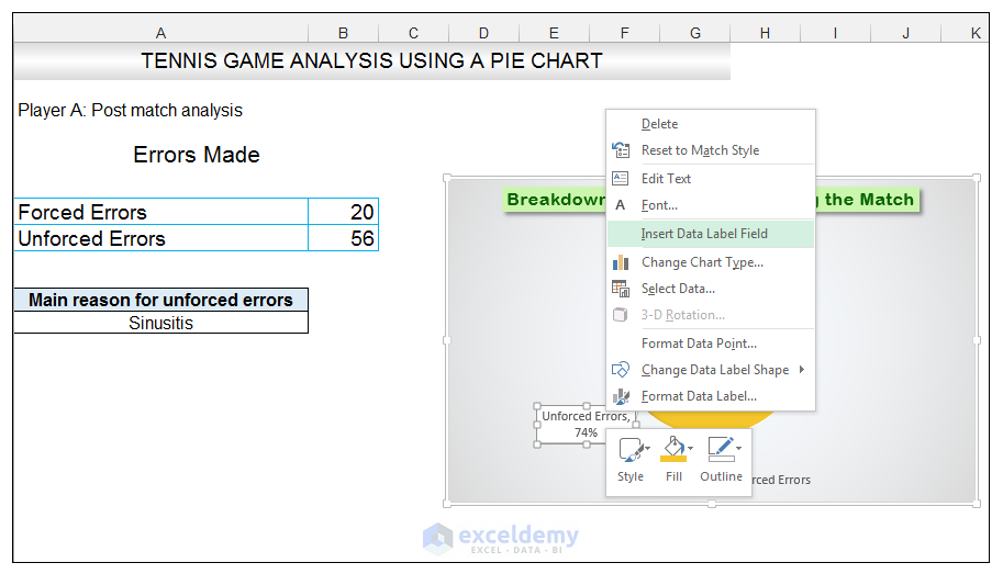
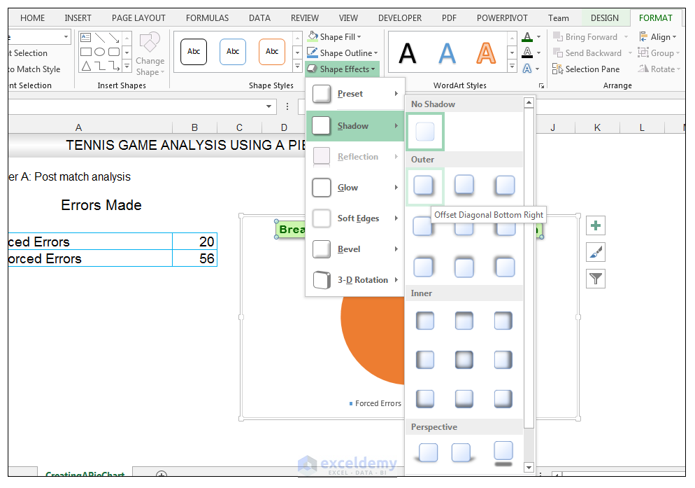
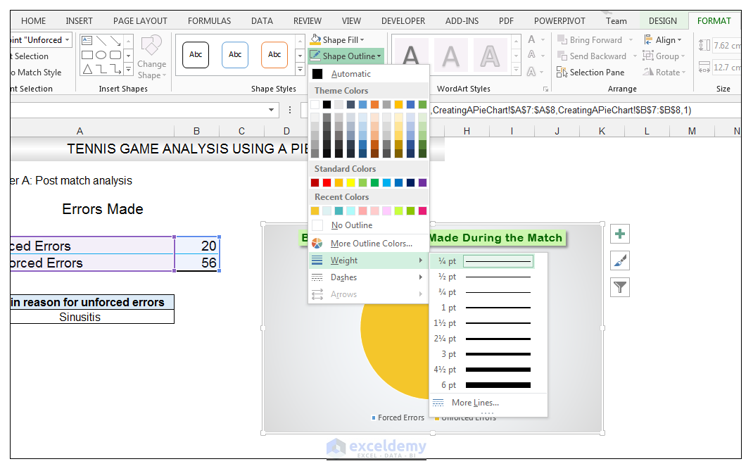
Data labels excel pie chart. How to Make a Pie Chart in Excel & Add Rich Data Labels to The Chart! Creating and formatting the Pie Chart 1) Select the data. 2) Go to Insert> Charts> click on the drop-down arrow next to Pie Chart and under 2-D Pie, select the Pie Chart, shown below. 3) Chang the chart title to Breakdown of Errors Made During the Match, by clicking on it and typing the new title. Resize Pie Chart Data Labels - Excel Charting & Graphing - Board ... 2. Type = in the formula bar and click on the. cell that you want to link to the label. Once linked you can explicitly control line. breaks using the CHAR worksheet function (e.g., ="long"&CHAR (10)&"label") or by using the. Alt+Enter key combination while entering the. label (i.e., type "long"; press Alt+Enter; excelunlocked.com › pie-of-pie-chart-in-excelPie of Pie Chart in Excel - Inserting, Customizing - Excel ... Jan 03, 2022 · In the above example, there were a total of 6 data points. The Parent Pie chart represents three of them i.e Facebook, Youtube, and Instagram while the fourth data point named “Other” splits into a subset Pie chart that represents the rest of the three data points i.e Zee, Linkedin, and Hotstar. How to fix wrapped data labels in a pie chart - Sage Intelligence Right click on the data label and select Format Data Labels. 2. Select Text Options > Text Box > and un-select Wrap text in shape. 3. The data labels resize to fit all the text on one line. 4. Alternatively, by double-clicking a data label, the handles can be used to resize the label to wrap words as desired. This can be done on all data labels ...

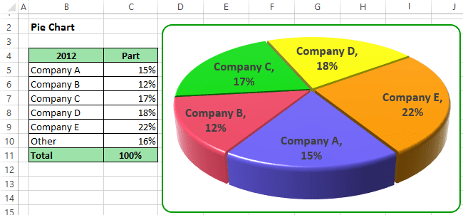
How to Create a Pie Chart in Excel | Smartsheet Enter data into Excel with the desired numerical values at the end of the list. Create a Pie of Pie chart. Double-click the primary chart to open the Format Data Series window. Click Options and adjust the value for Second plot contains the last to match the number of categories you want in the "other" category. Multiple data labels (in separate locations on chart) Re: Multiple data labels (in separate locations on chart) You can do it in a single chart. Create the chart so it has 2 columns of data. At first only the 1 column of data will be displayed. Move that series to the secondary axis. You can now apply different data labels to each series. Attached Files 819208.xlsx‎ (13.8 KB, 264 views) Download Office: Display Data Labels in a Pie Chart - Tech-Recipes 3. In the Chart window, choose the Pie chart option from the list on the left. Next, choose the type of pie chart you want on the right side. 4. Once the chart is inserted into the document, you will notice that there are no data labels. To fix this problem, select the chart, click the plus button near the chart's bounding box on the right ... Display data point labels outside a pie chart in a paginated report ... Create a pie chart and display the data labels. Open the Properties pane. On the design surface, click on the pie itself to display the Category properties in the Properties pane. Expand the CustomAttributes node. A list of attributes for the pie chart is displayed. Set the PieLabelStyle property to Outside. Set the PieLineColor property to Black.

Pie Chart in Excel - Inserting, Formatting, Filters, Data Labels To add Data Labels, Click on the + icon on the top right corner of the chart and mark the data label checkbox. You can also unmark the legends as we will add legend keys in the data labels. We can also format these data labels to show both percentage contribution and legend:- Right click on the Data Labels on the chart. Creating Pie Chart and Adding/Formatting Data Labels (Excel) Creating Pie Chart and Adding/Formatting Data Labels (Excel) Edit titles or data labels in a chart - support.microsoft.com On a chart, click one time or two times on the data label that you want to link to a corresponding worksheet cell. The first click selects the data labels for the whole data series, and the second click selects the individual data label. Right-click the data label, and then click Format Data Label or Format Data Labels. How to Edit Pie Chart in Excel (All Possible Modifications) How to Edit Pie Chart in Excel 1. Change Chart Color 2. Change Background Color 3. Change Font of Pie Chart 4. Change Chart Border 5. Resize Pie Chart 6. Change Chart Title Position 7. Change Data Labels Position 8. Show Percentage on Data Labels 9. Change Pie Chart's Legend Position 10. Edit Pie Chart Using Switch Row/Column Button 11.

How to Make Labels the Same Color as the Pies in Pie Chart - ExcelNotes

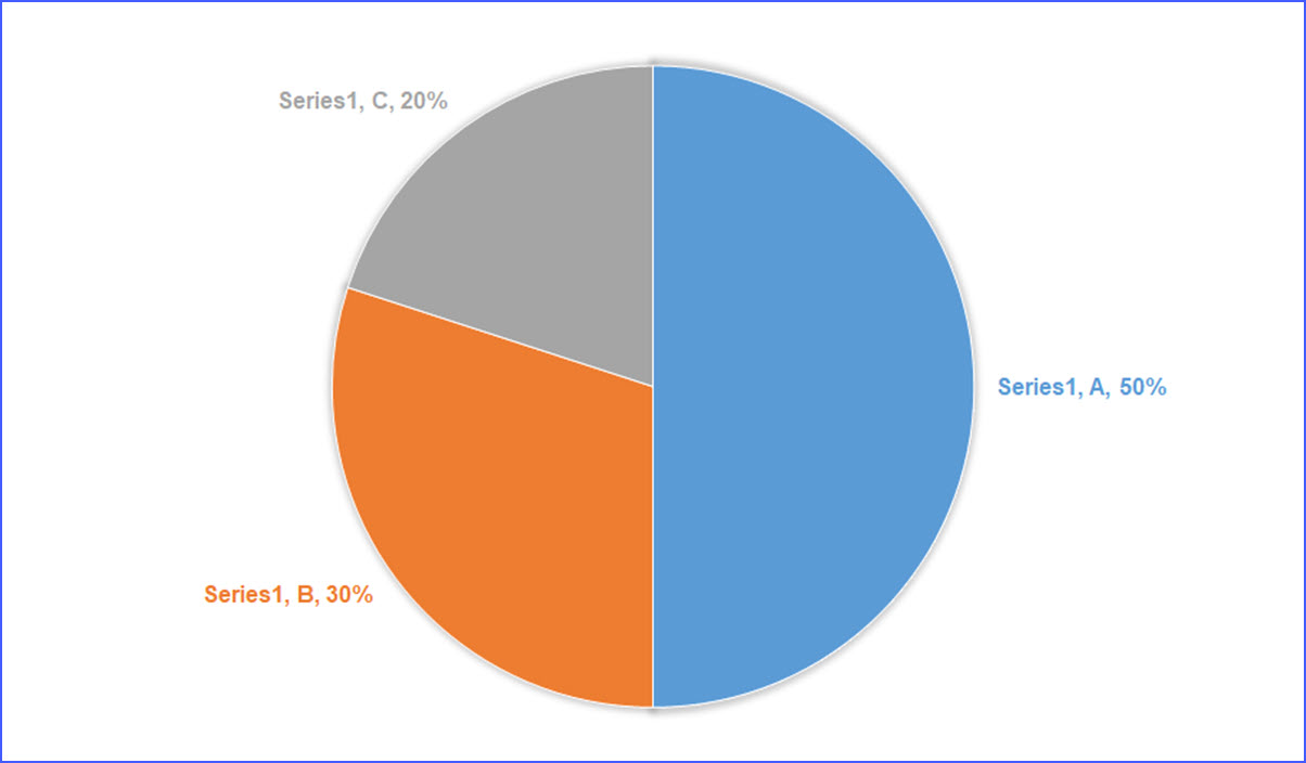
support.microsoft.com › en-us › officeAdd or remove data labels in a chart - support.microsoft.com Data labels make a chart easier to understand because they show details about a data series or its individual data points. For example, in the pie chart below, without the data labels it would be difficult to tell that coffee was 38% of total sales. Depending on what you want to highlight on a chart, you can add labels to one series, all the ...

Create a Pie Chart in Excel - Easy Excel Tutorial

Create a Pie Chart in Excel - Easy Steps / Become a Pro Select the pie chart. 9. Click the + button on the right side of the chart and click the check box next to Data Labels. 10. Click the paintbrush icon on the right side of the chart and change the color scheme of the pie chart. Result: 11. Right click the pie chart and click Format Data Labels. 12.

Nested donut chart (also known as Multi-level doughnut chart, Multi-series doughnut chart ...

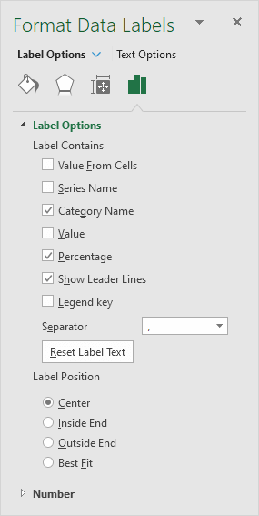
support.microsoft.com › en-us › officeChange the format of data labels in a chart To get there, after adding your data labels, select the data label to format, and then click Chart Elements > Data Labels > More Options. To go to the appropriate area, click one of the four icons ( Fill & Line , Effects , Size & Properties ( Layout & Properties in Outlook or Word), or Label Options ) shown here.

Microsoft Excel Tutorials: Add Data Labels to a Pie Chart

How to Make a Pie Chart in Excel (Only Guide You Need) To add labels to the slices of the pie chart do the following. 1 st select the pie chart and press on to the "+" shaped button which is actually the Chart Elements option Then put a tick mark on the Data Labels You will see that the data labels are inserted into the slices of your pie chart.

How to Make a Pie Chart in Excel & Add Rich Data Labels to The Chart!

› pie-chart-in-excelPie Chart in Excel | How to Create Pie Chart | Step-by-Step ... Large data can be presented by using the Pie Chart in Excel. With the help of each slice bar, we can easily compare one with another. Easy and no need to explain it to the end-user. It is understandable by any means. Disadvantages: Fitting data labels in the case of smaller values is very difficult. It will overlap with other data labels.

How to Make a Pie Chart in Excel & Add Rich Data Labels to The Chart!

Multiple Data Labels on a Pie Chart | MrExcel Message Board This table includes: Column 1 - shipment name Column 2 - shipment cost Column 3 - shipment weight I have created a pie chart from this table, which covers the first two columns. Displayed next to each slice is a label with the shipment name, shipment cost, and percent share of the pie.

How to create pie of pie or bar of pie chart in Excel?

Inserting Data Label in the Color Legend of a pie chart Inserting Data Label in the Color Legend of a pie chart. Hi, I am trying to insert data labels (percentages) as part of the side colored legend, rather than on the pie chart itself, as displayed on the image below. Does Excel offer that option and if so, how can i go about it?