38 how to format data labels in excel charts
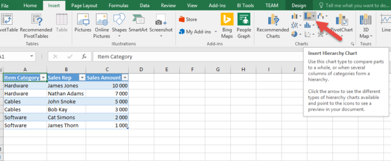
How to format axis labels as thousands/millions in Excel? Right click at the axis you want to format its labels as thousands/millions, select Format Axisin the context menu. 2. In the Format Axisdialog/pane, click Number tab, then in theCategorylist box, select Custom, and type[>999999] #,,"M";#,"K"into Format Codetext box, and click Addbutton to add it toTypelist. See screenshot: 3. How to Create Excel Charts (Column or Bar) with Conditional Formatting Step #2: Set up a column chart. Having gathered all the chart data, set up a simple column chart—or a bar chart as an alternative:. Highlight all the chart data except for the columns containing the actual values and the rules by holding down the Ctrl key (A4:A12 and C4:D12).; Go to the Insert tab.; Select "Insert Column or Bar Chart. Choose "Clustered Column/Clustered Bar.
How to Customize Your Excel Pivot Chart Data Labels - dummies To add data labels, just select the command that corresponds to the location you want. To remove the labels, select the None command. If you want to specify what Excel should use for the data label, choose the More Data Labels Options command from the Data Labels menu. Excel displays the Format Data Labels pane.

How to format data labels in excel charts
How to change chart axis labels' font color and size in Excel? Just click to select the axis you will change all labels' font color and size in the chart, and then type a font size into the Font Size box, click the Font color button and specify a font color from the drop down list in the Font group on the Home tab. See below screen shot: How to hide zero data labels in chart in Excel? - ExtendOffice In the Format Data Labelsdialog, Click Numberin left pane, then selectCustom from the Categorylist box, and type #""into the Format Codetext box, and click Addbutton to add it to Typelist box. See screenshot: 3. Click Closebutton to close the dialog. Then you can see all zero data labels are hidden. How to Change Excel Chart Data Labels to Custom Values? First add data labels to the chart (Layout Ribbon > Data Labels) Define the new data label values in a bunch of cells, like this: Now, click on any data label. This will select "all" data labels. Now click once again. At this point excel will select only one data label.
How to format data labels in excel charts. Add / Move Data Labels in Charts - Excel & Google Sheets Adding Data Labels Click on the graph Select + Sign in the top right of the graph Check Data Labels Change Position of Data Labels Click on the arrow next to Data Labels to change the position of where the labels are in relation to the bar chart Final Graph with Data Labels How to create Custom Data Labels in Excel Charts Two ways to do it. Click on the Plus sign next to the chart and choose the Data Labels option. We do NOT want the data to be shown. To customize it, click on the arrow next to Data Labels and choose More Options … Unselect the Value option and select the Value from Cells option. Choose the third column (without the heading) as the range. Change the format of data labels in a chart To get there, after adding your data labels, select the data label to format, and then click Chart Elements > Data Labels > More Options. To go to the appropriate area, click one of the four icons ( Fill & Line, Effects, Size & Properties ( Layout & Properties in Outlook or Word), or Label Options) shown here. Excel Charts - Aesthetic Data Labels - Tutorials Point Step 1 − Right-click a data label and then click Format Data Label. The Format Pane - Format Data Label appears. Step 2 − Click the Fill & Line icon. The options for Fill and Line appear below it. Step 3 − Under FILL, Click Solid Fill and choose the color.
How to add or move data labels in Excel chart? - ExtendOffice In Excel 2013 or 2016. 1. Click the chart to show the Chart Elements button . 2. Then click the Chart Elements, and check Data Labels, then you can click the arrow to choose an option about the data labels in the sub menu. See screenshot: In Excel 2010 or 2007. 1. click on the chart to show the Layout tab in the Chart Tools group. See ... How to Insert Axis Labels In An Excel Chart | Excelchat We will again click on the chart to turn on the Chart Design tab. We will go to Chart Design and select Add Chart Element. Figure 6 - Insert axis labels in Excel. In the drop-down menu, we will click on Axis Titles, and subsequently, select Primary vertical. Figure 7 - Edit vertical axis labels in Excel. Now, we can enter the name we want ... How to create a Geographic map chart in Microsoft Excel Create the map chart. When you're ready to create the map chart, select your data by dragging it across cells, open the "Insert" tab, and move to the "Charts" section of the ribbon. Click on the "Maps" dropdown menu and choose "Full Map". Your newly created chart will appear directly on your sheet with your assigned data. excel - Formatting chart data labels with VBA - Stack Overflow Here's the code so far: Sub FixLabels (whichchart As String) Dim cht As Chart Dim i, z As Variant Dim seriesname, seriesfmt As String Dim seriesrng As Range Set cht = Sheets ("Dashboard").ChartObjects (whichchart).Chart For i = 1 To cht.SeriesCollection.Count If cht.SeriesCollection (i).name = "#N/D" Then cht.SeriesCollection (i).DataLabels ...
Custom Chart Data Labels In Excel With Formulas Follow the steps below to create the custom data labels. Select the chart label you want to change. In the formula-bar hit = (equals), select the cell reference containing your chart label's data. In this case, the first label is in cell E2. Finally, repeat for all your chart laebls. Format Data Labels in Excel- Instructions - TeachUcomp, Inc. To do this, click the "Format" tab within the "Chart Tools" contextual tab in the Ribbon. Then select the data labels to format from the "Chart Elements" drop-down in the "Current Selection" button group. Then click the "Format Selection" button that appears below the drop-down menu in the same area. 【How-to】How to edit legend in excel - Howto.org Click the chart, and then click the Chart Design tab. Click Add Chart Element and select Data Labels, and then select a location for the data label option. Note: The options will differ depending on your chart type. If you want to show your data label inside a text bubble shape, click Data Callout. Add a DATA LABEL to ONE POINT on a chart in Excel All the data points will be highlighted. Click again on the single point that you want to add a data label to. Right-click and select ' Add data label '. This is the key step! Right-click again on the data point itself (not the label) and select ' Format data label '. You can now configure the label as required — select the content of ...
Format Number Options for Chart Data Labels in Excel 2011 for Mac
Custom Data Labels with Colors and Symbols in Excel Charts - [How To] To apply custom format on data labels inside charts via custom number formatting, the data labels must be based on values. You have several options like series name, value from cells, category name. But it has to be values otherwise colors won't appear. Symbols issue is quite beyond me.

Microsoft Excel Tutorials: The Chart Layout Panels
How to add data labels from different column in an Excel chart? Right click the data series, and select Format Data Labels from the context menu. 3. In the Format Data Labels pane, under Label Options tab, check the Value From Cells option, select the specified column in the popping out dialog, and click the OK button. Now the cell values are added before original data labels in bulk. 4.
How to create a Tree Map chart in Excel 2016 | Sage Intelligence
Change axis labels in a chart - support.microsoft.com On the Character Spacing tab, choose the spacing options you want. To change the format of numbers on the value axis: Right-click the value axis labels you want to format. Click Format Axis. In the Format Axis pane, click Number. Tip: If you don't see the Number section in the pane, make sure you've selected a value axis (it's usually the ...

How to Add Data Labels to your Excel Chart in Excel 2013 - YouTube
How to Use Cell Values for Excel Chart Labels Select the chart, choose the "Chart Elements" option, click the "Data Labels" arrow, and then "More Options." Uncheck the "Value" box and check the "Value From Cells" box. Select cells C2:C6 to use for the data label range and then click the "OK" button. The values from these cells are now used for the chart data labels.
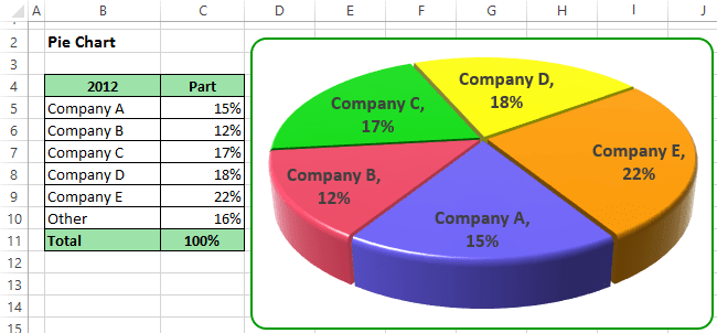
Excel 3-D Pie charts - Microsoft Excel 2013
Add or remove data labels in a chart - support.microsoft.com Right-click the data series or data label to display more data for, and then click Format Data Labels. Click Label Options and under Label Contains, select the Values From Cells checkbox. When the Data Label Range dialog box appears, go back to the spreadsheet and select the range for which you want the cell values to display as data labels.

Microsoft Excel Tutorials: The Chart Layout Panels
Edit titles or data labels in a chart - support.microsoft.com The first click selects the data labels for the whole data series, and the second click selects the individual data label. Right-click the data label, and then click Format Data Label or Format Data Labels. Click Label Options if it's not selected, and then select the Reset Label Text check box. Top of Page
![Custom Data Labels with Colors and Symbols in Excel Charts - [How To] - PakAccountants.com](https://pakaccountants.b-cdn.net/wp-content/uploads/2014/09/data-label-chart-8.gif)
Custom Data Labels with Colors and Symbols in Excel Charts - [How To] - PakAccountants.com
How to Create a Bar Chart With Labels Above Bars in Excel In the Format Data Labels pane, under Label Options selected, set the Label Position to Inside End. 16. Next, while the labels are still selected, click on Text Options, and then click on the Textbox icon. 17. Uncheck the Wrap text in shape option and set all the Margins to zero. The chart should look like this: 18.

34 Label Chart In Excel - Labels Database 2020
How to Find, Highlight, and Label a Data Point in Excel Scatter Plot? By default, the data labels are the y-coordinates. Step 3: Right-click on any of the data labels. A drop-down appears. Click on the Format Data Labels… option. Step 4: Format Data Labels dialogue box appears. Under the Label Options, check the box Value from Cells . Step 5: Data Label Range dialogue-box appears.

Excel Dashboard Templates How-to Use Data Labels from a Range in an Excel Chart - Excel ...
How do you change the horizontal axis labels in Excel? Click the data series or chart. In the upper right corner, next to the chart, click Add Chart Element > Data Labels. To change the location, click the arrow, and choose an option. If you want to show your data label inside a text bubble shape, click Data Callout.

Elements of an Excel Chart | ExcelDemy.com
How to Change Excel Chart Data Labels to Custom Values? First add data labels to the chart (Layout Ribbon > Data Labels) Define the new data label values in a bunch of cells, like this: Now, click on any data label. This will select "all" data labels. Now click once again. At this point excel will select only one data label.
34 Data Label In Excel Chart - Labels For Your Ideas
How to hide zero data labels in chart in Excel? - ExtendOffice In the Format Data Labelsdialog, Click Numberin left pane, then selectCustom from the Categorylist box, and type #""into the Format Codetext box, and click Addbutton to add it to Typelist box. See screenshot: 3. Click Closebutton to close the dialog. Then you can see all zero data labels are hidden.
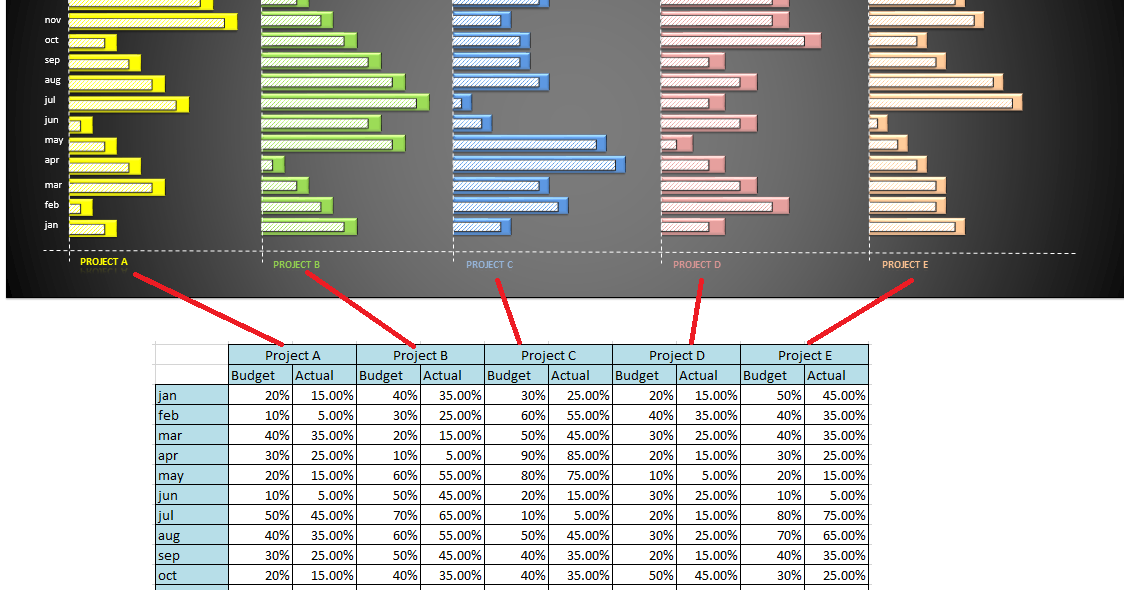
Do My Excel Blog: How to design a multiple clustered bar chart series in Excel
How to change chart axis labels' font color and size in Excel? Just click to select the axis you will change all labels' font color and size in the chart, and then type a font size into the Font Size box, click the Font color button and specify a font color from the drop down list in the Font group on the Home tab. See below screen shot:

Do My Excel Blog: How to design a multiple clustered bar chart series in Excel
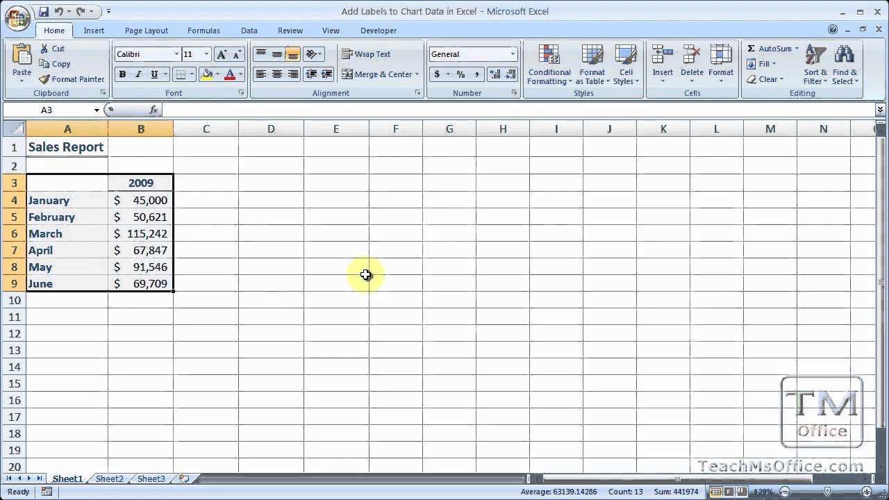
Add Labels to Chart Data in Excel - YouTube

How to Add Data Labels in Excel - Excelchat | Excelchat
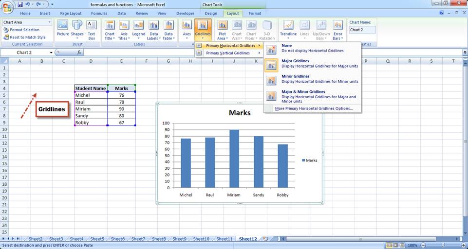
Basic Excel Chart Formatting - MS Excel Charting Tutorial Part 4 | Vertical Horizons
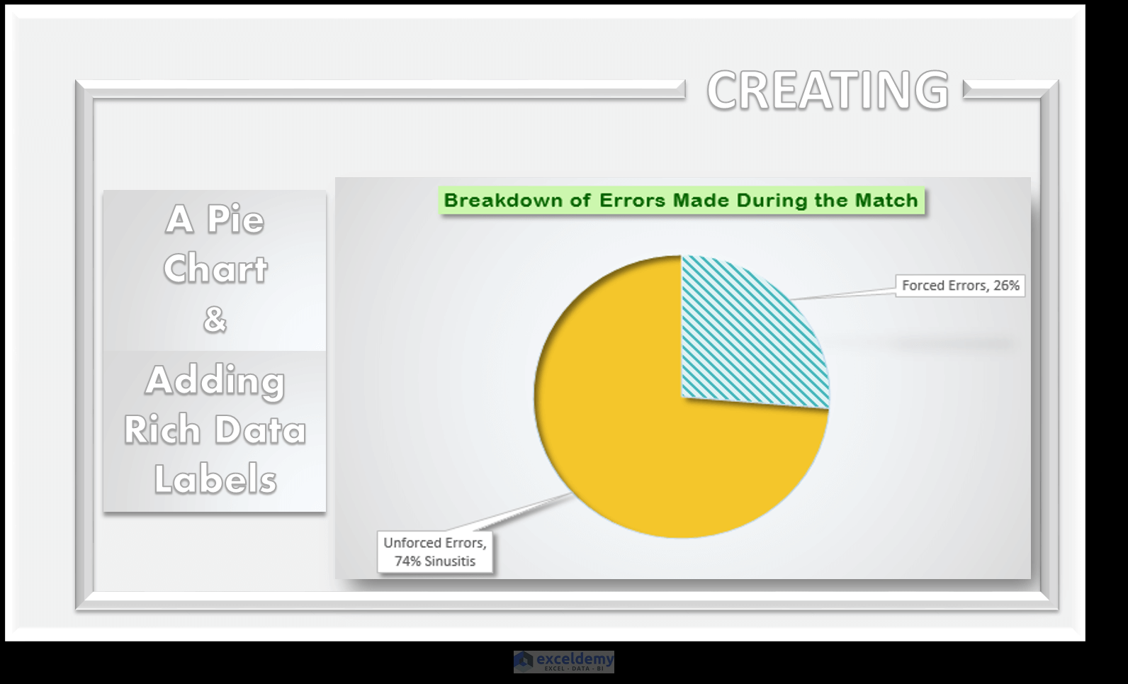
How to Make a Pie Chart in Excel & Add Rich Data Labels to The Chart!
Post a Comment for "38 how to format data labels in excel charts"