42 excel 2013 data labels
Change the format of data labels in a chart To get there, after adding your data labels, select the data label to format, and then click Chart Elements > Data Labels > More Options. To go to the appropriate area, click one of the four icons ( Fill & Line, Effects, Size & Properties ( Layout & Properties in Outlook or Word), or Label Options) shown here. Adding rich data labels to charts in Excel 2013 ... You can do this by adjusting the zoom control on the bottom right corner of Excel's chrome. Then, select the value in the data label and hit the right-arrow key on your keyboard. The story behind the data in our example is that the temperature increased significantly on Wednesday and that appeared to help drive up business at the lemonade stand.
Adding Data Labels to Your Chart - Excel ribbon tips To add data labels in Excel 2013 or Excel 2016, follow these steps: Activate the chart by clicking on it, if necessary. Make sure the Design tab of the ribbon is displayed. (This will appear when the chart is selected.) Click the Add Chart Element drop-down list. Select the Data Labels tool.
Excel 2013 data labels
How to hide zero data labels in chart in Excel? - ExtendOffice Note: In Excel 2013, you can right click the any data label and select Format Data Labels to open the Format Data Labels pane; then click Number to expand its option; next click the Category box and select the Custom from the drop down list, and type #"" into the Format Code text box, and click the Add button. Custom Data Labels with Colors and Symbols in Excel Charts ... The basic idea behind custom label is to connect each data label to certain cell in the Excel worksheet and so whatever goes in that cell will appear on the chart as data label. So once a data label is connected to a cell, we apply custom number formatting on the cell and the results will show up on chart also. Add a Data Callout Label to Charts in Excel 2013 In the upper right corner, next to your chart, click the Chart Elements button (plus sign), and then click Data Labels. A right pointing arrow will appear, click on this arrow to view the submenu. Select Data Callout. Once the Data Callout Labels have been added, you can re-position them by clicking on their borders and dragging to a new position.
Excel 2013 data labels. How to Customize Chart Elements in Excel 2013 - dummies To add data labels to your selected chart and position them, click the Chart Elements button next to the chart and then select the Data Labels check box before you select one of the following options on its continuation menu: Center to position the data labels in the middle of each data point. Inside End to position the data labels inside each ... Change the format of data labels in a chart To get there, after adding your data labels, select the data label to format, and then click Chart Elements > Data Labels > More Options. To go to the appropriate area, click one of the four icons ( Fill & Line, Effects, Size & Properties ( Layout & Properties in Outlook or Word), or Label Options) shown here. Values From Cell: Missing Data Labels Option in Excel 2013? When a chart created in 2013 using the "Values from Cell" data label option is opened with any earlier version of Excel, the data labels will show as " [CELLRANGE]". If you want to ensure that data labels survive different generations of Excel, you need to revert to the old technique: Insert data labels Edit each individual data label Values From Cell: Missing Data Labels Option in Excel 2013? A couple articles refer to formatting data labels and values to have it pull what you want. I have a feeling they used a 3rd party ad-in like tech-cell or some such and because I don't have the add in its not happy. Im following the blog reference here: Adding rich data labels to charts in Excel 2013 - Office Blogs
Creating a chart with dynamic labels - Microsoft Excel 2013 Excel 2013 365 2016 This tip shows how to create dynamically updated chart labels that depend on value or other cells. The trick of this chart is to show data from specific cells in the chart labels. Edit titles or data labels in a chart - support.microsoft.com The first click selects the data labels for the whole data series, and the second click selects the individual data label. Right-click the data label, and then click Format Data Label or Format Data Labels. Click Label Options if it's not selected, and then select the Reset Label Text check box. Top of Page How to Print Labels From Excel - Lifewire Choose Start Mail Merge > Labels . Choose the brand in the Label Vendors box and then choose the product number, which is listed on the label package. You can also select New Label if you want to enter custom label dimensions. Click OK when you are ready to proceed. Connect the Worksheet to the Labels How to Add Data Labels in Excel - Excelchat | Excelchat In Excel 2013 and the later versions we need to do the followings; Click anywhere in the chart area to display the Chart Elements button Figure 5. Chart Elements Button Click the Chart Elements button > Select the Data Labels, then click the Arrow to choose the data labels position. Figure 6. How to Add Data Labels in Excel 2013 Figure 7.
How to create Custom Data Labels in Excel Charts Two ways to do it. Click on the Plus sign next to the chart and choose the Data Labels option. We do NOT want the data to be shown. To customize it, click on the arrow next to Data Labels and choose More Options …. Unselect the Value option and select the Value from Cells option. Choose the third column (without the heading) as the range. Excel 2013 - Line Chart Data Labels - Data Callout submenu ... In one of them I can see the Data Callout submenu which allows me to specific content for data labels to appear at specific points on the line-graph. The "label options/label contains" area in the formatting box then includes a "value from cells" tickbox that allows me specify that the values that come from a specific excel cell range. Create and print mailing labels for an address list in Excel Column names in your spreadsheet match the field names you want to insert in your labels. All data to be merged is present in the first sheet of your spreadsheet. Postal code data is correctly formatted in the spreadsheet so that Word can properly read the values. The Excel spreadsheet to be used in the mail merge is stored on your local machine. Excel Tips n Tricks -Tip 8 (Applying Chart Data Labels ... Click on the plus symbol, the first icon, and check "Data Labels". Now you will see them added to your chart. You can also click on the right arrow on "Data Labels" and select where you want the data labels to be aligned, in other words center, right, top, bottom and so on. Picture 4 4. I modified the chart and axis titles to look good.
How to Add Labels to an Excel 2007 Chart - Bright Hub
How to Add Axis Labels in Excel 2013 - YouTube How to Add Axis Labels in Excel 2013For more tips and tricks, be sure to check out is a tutorial on how to add axis labels in E...

Enable or Disable Excel Data Labels at the click of a button - How To - PakAccountants.com
Custom Chart Labels Using Excel 2013 - MyExcelOnline View the Benchmark Chart using Excel 2013. DOWNLOAD EXCEL WORKBOOK. STEP 1: We added a % Variance column in our data and inserted symbols to show a negative and positive variance. ** You can see the tutorial of how this is done here **. STEP 2: In our graph we need to select the Sales chart and Right Click and choose Add Data Labels.
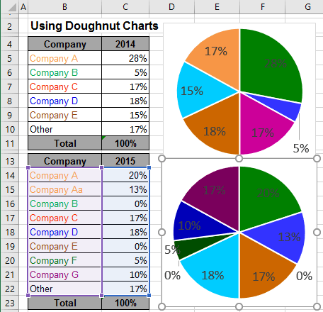
Using Pie Charts and Doughnut Charts in Excel
Add or remove data labels in a chart - support.microsoft.com To label one data point, after clicking the series, click that data point. In the upper right corner, next to the chart, click Add Chart Element > Data Labels. To change the location, click the arrow, and choose an option. If you want to show your data label inside a text bubble shape, click Data Callout.
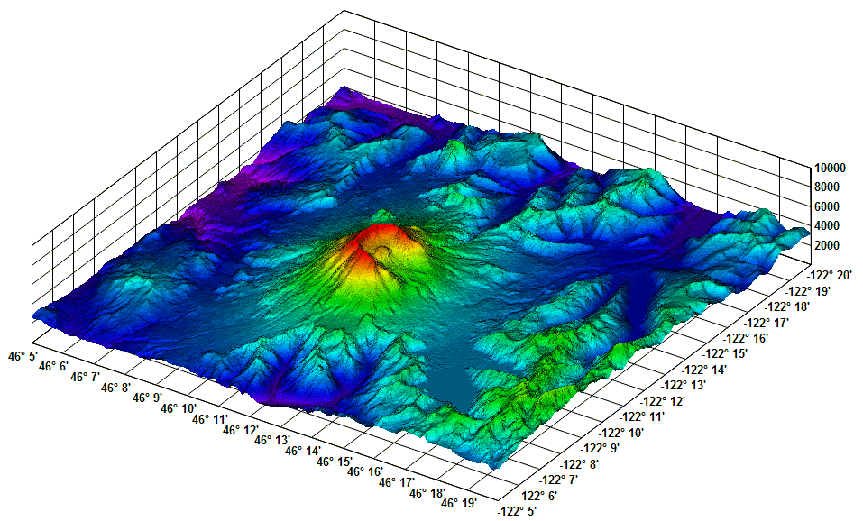
DPlot Graph Software for Scientists and Engineers
Quick Tip: Excel 2013 offers flexible data labels ... right-click and choose Insert Data Label Field. In the next dialog, select [Cell] Choose Cell. When Excel displays the source dialog, click the cell that contains the MIN () function, and click OK....

Enable or Disable Excel Data Labels at the click of a button - How To - PakAccountants.com
How to add data labels from different column in an Excel ... Right click the data series in the chart, and select Add Data Labels > Add Data Labels from the context menu to add data labels. 2. Click any data label to select all data labels, and then click the specified data label to select it only in the chart. 3.

How to Add Data Labels to an Excel 2010 Chart - dummies
Format Data Labels in Excel- Instructions - TeachUcomp, Inc. To format data labels in Excel, choose the set of data labels to format. To do this, click the "Format" tab within the "Chart Tools" contextual tab in the Ribbon. Then select the data labels to format from the "Chart Elements" drop-down in the "Current Selection" button group.

Excel chart not printing correctly - i have a simple excel file (office
Add a Data Callout Label to Charts in Excel 2013 In the upper right corner, next to your chart, click the Chart Elements button (plus sign), and then click Data Labels. A right pointing arrow will appear, click on this arrow to view the submenu. Select Data Callout. Once the Data Callout Labels have been added, you can re-position them by clicking on their borders and dragging to a new position.
MS Excel 2013: Display the fields in the Values Section in a single column in a pivot table
Custom Data Labels with Colors and Symbols in Excel Charts ... The basic idea behind custom label is to connect each data label to certain cell in the Excel worksheet and so whatever goes in that cell will appear on the chart as data label. So once a data label is connected to a cell, we apply custom number formatting on the cell and the results will show up on chart also.
31 Label Of Microsoft Excel
How to hide zero data labels in chart in Excel? - ExtendOffice Note: In Excel 2013, you can right click the any data label and select Format Data Labels to open the Format Data Labels pane; then click Number to expand its option; next click the Category box and select the Custom from the drop down list, and type #"" into the Format Code text box, and click the Add button.
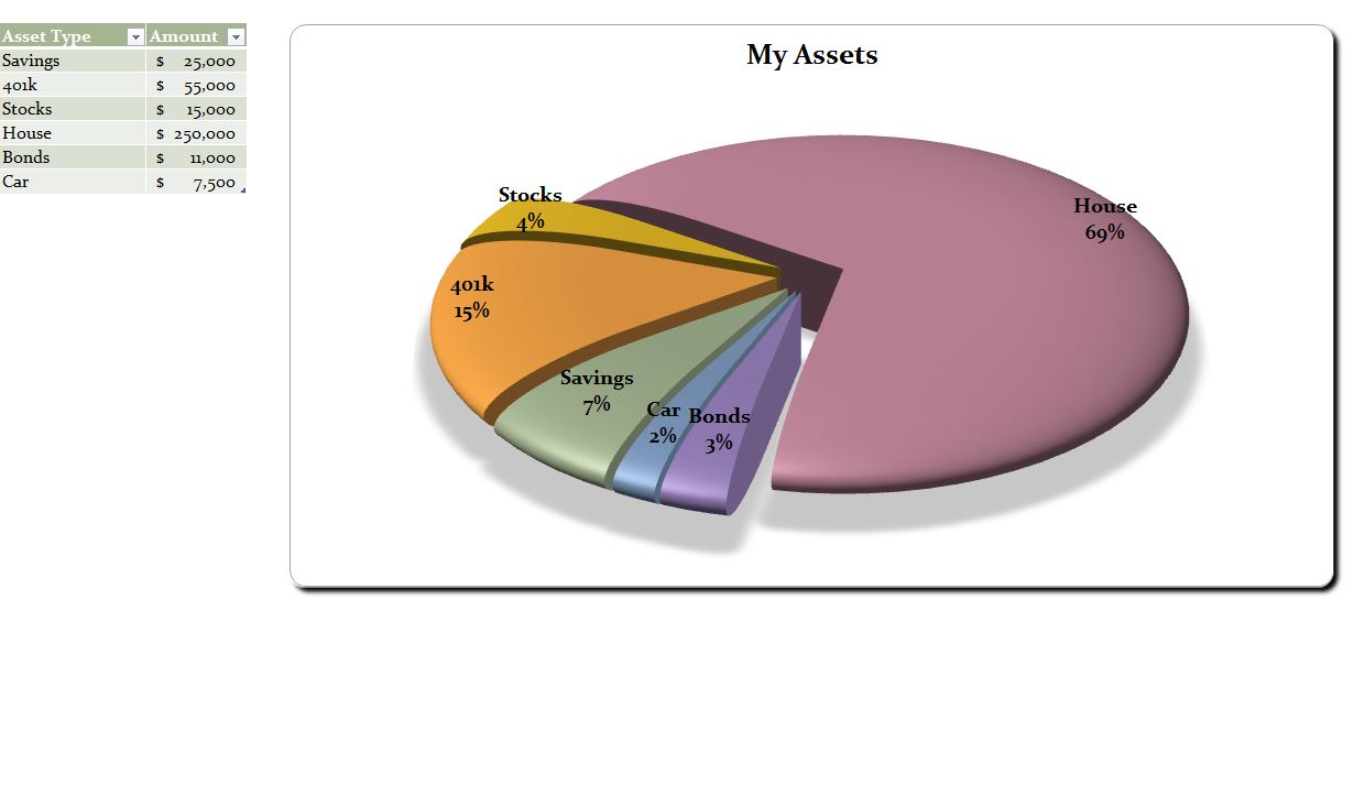
Excel Pie Chart | Pie Chart Excel

Format Data Labels in Excel- Instructions - TeachUcomp, Inc.

Advanced Graphs Using Excel : Creating dynamic range plots in Excel

How to Create a Chart in Microsoft Excel - TechSupport

How to Create a Pie Chart in Microsoft Excel

How to Create Multi-Category Chart in Excel - Excel Board

Excel 2013 Tutorial Formatting Data Labels Microsoft Training Lesson 28.6 - YouTube
Post a Comment for "42 excel 2013 data labels"